Equilibration
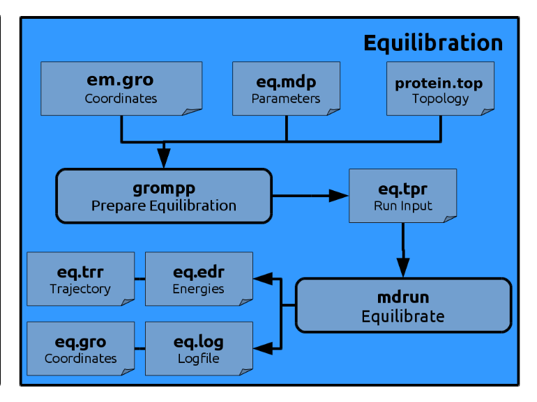
Our energy minimized system now needs an equilibration MD simulation to further relax the system.
The water molecules that we created as a crystal lattice can then rearrange around the solute.
As we do not want the protein to move significantly during the equilibration phase,
we will restrain it with harmonic forces to its initial position.
This is done by defining the macro POSRES in the file eq.mdp
and making use of kigaki_posre.itp, which is achieved by the following statement in kigaki.top:
        ; Include Position restraint file

        #ifdef POSRES

        #include "kigaki_posre.itp"

        #endif
grompp to insert the harmonic restraining forces into the *.tpr file.
In the parameter file (eq.mdp), we choose the integrator md,
which is acutally a leap-frog verlet integrator to compute the position updates at every timestep from the previous timestep.
We set the timestep length to 2 femtoseconds.
In addition to the parameters you already know from the energy minimization,
we now use a thermostat and a barostat to make the temperature and pressure fluctuate around room temperature
and atmospheric pressure.
We instruct grompp to generate new velocities from a Boltzmann distribution at room
temperature.
Finally we set constraints on all bonds.
This will ensure that bonds will not deviate too much from their equilibrium positions,
even if we increase the timestep beyond the point were it can resolve bond vibrations properly.
As we do not expect bond vibrations to influence the overall dynamics of our system significantly,
this speeds up the simulation quite a bit without sacrificying much accuracy.
Consult the Gromacs manual for a detailed explanation.
Generate the run input file:
gmx grompp -f eq.mdp -po eq.out.mdp -c em.gro -r em.gro -t em.trr -p kigaki.top -o eq.tpr
gmx mdrun -v -deffnm eq >& eq.out &
& at the end ensures that the command, i.e., the simulation will be run in the background.
All output is written to the file eq.out.
While the simulation is running you can monitor the progress with the command:
tail -f eq.out
eq.log).
Once the simulation is done, you should control that the results are not unphysical.
Despite visual inspection you can again have a look at the energy output (eq.edr)
with gmx energy to make sure that, for example, the temperature fluctuates around the
desired value and the density is not decreasing,
which would indicate that your system is blowing up.
Once the simulation is done, convert it again to make all molecules whole and transformed to the central simulation box:
gmx trjconv -f eq.xtc -s eq.tpr -o eq_centered.xtc -ur compact -pbc mol -centergmx trjconv -f eq.xtc -s eq.tpr -o eq_centered.pdb -ur compact -pbc mol -center -dump 0
-dump 0 flag creates a pdb file that contains the coordinates of the peptide at time t=0.
Open the trajectory in VMD as you did after the energy minimization.
You should see a protein that is hardly moving, at least not changing its overall shape,
and freely moving water molecules and ions.
To get a little more used to VMD try the following:
Open the Representations menu that you find in the
Graphics menu of the VMD Main Window.
Change the Selection to protein
and the Drawing Method to Licorice.
Now switch to the Trajectory tab and set the
Trajectory Smoothing Window Size to 5.
In effect, each frame you see in the Graphics window is now the average over 5 frames and the protein movement will
appear much smoother.
Now create a new Representation.
Enter the selection text same residue as (within 5 of protein).
Set the Drawing Method to Lines and the
Trajectory Smoothing Window Size again to 5 or higher.
You can now observe the water molecules that are initially close to the protein
(in a 5 Ångstrom shell around it) diffusing away.
Alternatively you can set the option Update Selection Every Frame
in the Representations window’s Trajectory tab.
This will show you the water molecules that are close to the protein in each frame.
If you are certain that your equilibration looks fine, move on to the production MD stage.

