Analysis

Principal component analysis (PCA)

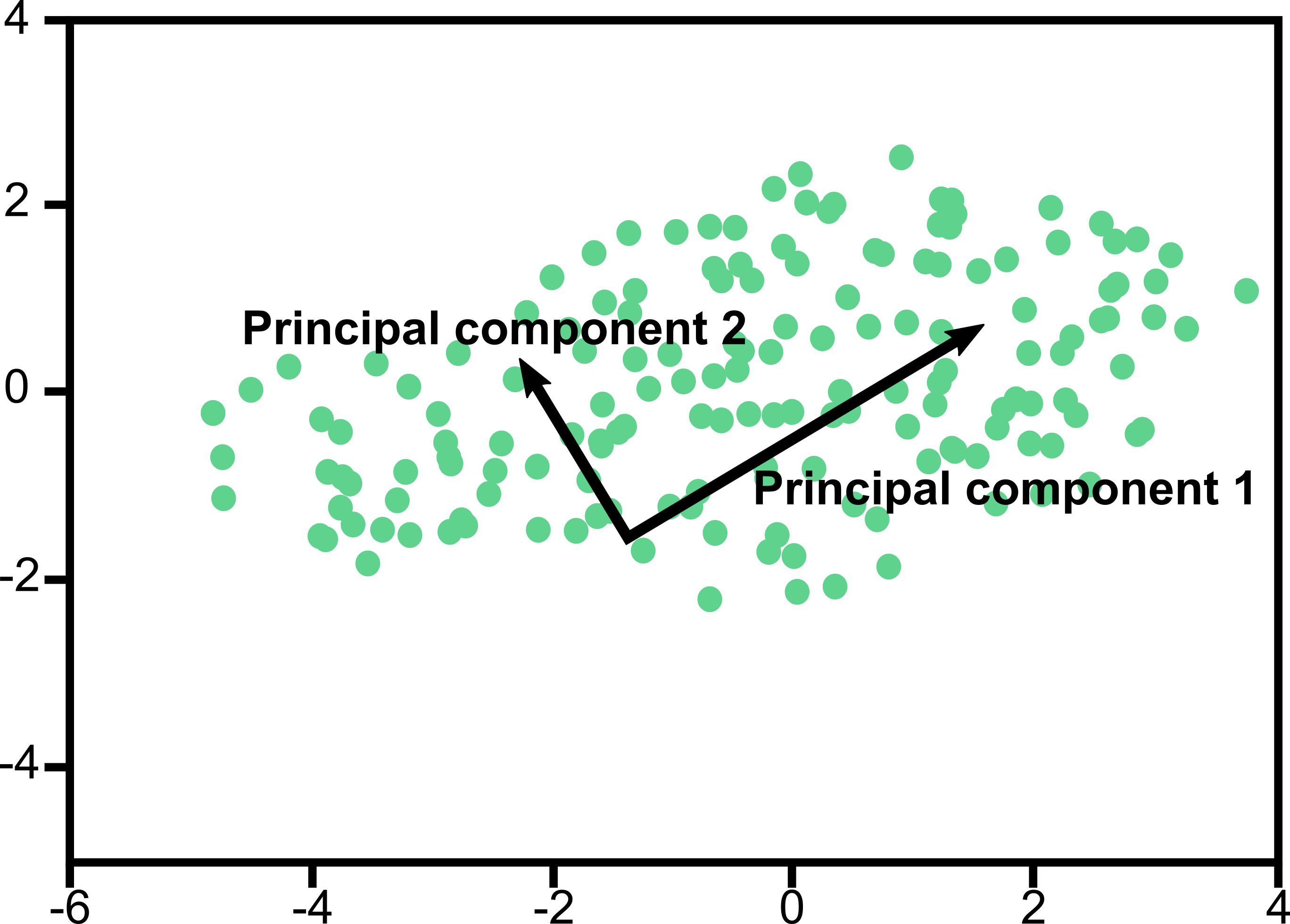
Principal component analysis is also called covariance analysis or essential dynamics analysis. Similar to clustering, it can help us identify the important parts of large trajectories. PCA in particular identifies the largest motions that take place in the system:

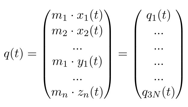
Our trajectory, as it is, uses the Cartesian xyz coordinates of all N atoms, so any motion of the protein needs to be described in a dimension of 3N, which is pretty unwieldy. Therefore, we will define our coordinates as a vector q(t), with m_i denoting the mass of the ith atom, and x_i(t) the x coordinate of atom i at time t:

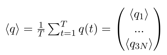
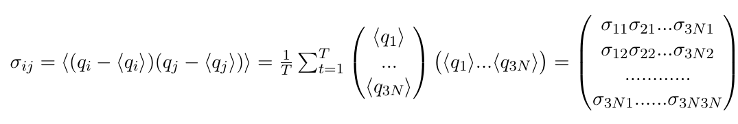
Any other ordering of elements is also fine, as long as we stay consistent, which is why the selected group in the GROMACS function has to stay the same. Now, we can calculate the averages of each of these elements, where T stands for the number of frames in our trajectory:

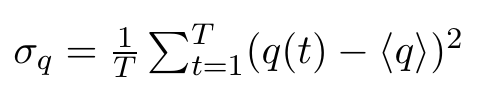
Note that all of these entries are plain numbers. Imagine a little histogram of atom 1's x-positions, with an average value < q₁ > and a variance σ₁₁. Now, We have reduced 3N little histograms to 3N averages. Additionally, we want to have the variance, which is defined as:

and would be a 3N dimensional vector (of plain numbers). These will appear on the diagonal of our covariance matrix. The off-diagonal elements, however, are the actual covariances, where positions of two DIFFERENT atoms are correlated. And we want to correlate ALL atoms with ALL other atoms, which we can write as a column vector multiplied with a row vector, resulting in a 3Nx3N dimensional matrix:

All of these entries are still numbers. A large positive number means that the two atoms move along this axis in a highly correlated fashion, or that this atom moves along both its axes in a highly correlated fashion. Imagine a protein with an extended "arm" that waves up and down. A large negative number indicates the motions are anticorrelated. Imagine a protein where one "arm" moves up while the other "arm" moves down. A zero can mean that the motions are completely uncorrelated.
By diagonalizing σ, we obtain 3N eigenvectors v⁽ⁱ⁾ and eigenvalues λ_i with

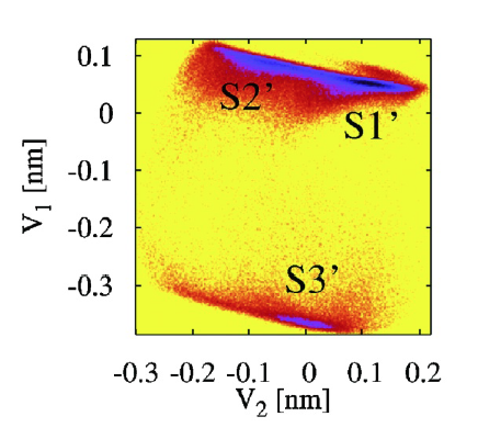
The eigenvectors and eigenvalues of σ yield the modes of collective motion and their amplitudes. The principal components (PCs) or eigenvectors (eigv) can then be used, for example, to represent the free energy surface. From the above equation we see that, e.g., the first three components v₁⁽ⁱ⁾, v₂⁽ⁱ⁾ and v₃⁽ⁱ⁾ of the eigenvector v⁽ⁱ⁾ reflect the influence of the x, y and z coordinates of the first atom on the i-th PC.

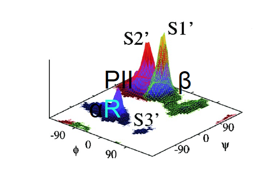
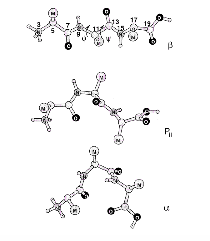
Example: Free energy surface of Ala3 in water as obtained from a 100 ns MD simulation using PCA, including the (φ,ψ) distribution pertaining to the labeled energy minima:

1. Building the covarience matrix:

gmx covar builds and diagonalizes the covariance matrix. Only select the backbone for the calculation as we are interested in motions of the whole protein but not of the sidechains.

gmx covar -f md_protein.xtc -s md_protein.tpr (Selection: "Backbone")

which produces the files eigenvec.trr and eigenval.xvg. By diagonalizing σ, we obtain 3N eigenvectors v_i (dimension is still 3N) and eigenvalues λ_i. These eigenvectors can be our new basis.

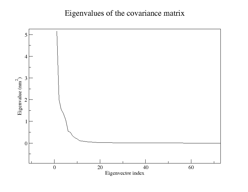
Think of our previous conformational space as a 3N-dimensional cube, where all our little histograms live as clouds of dots. Eigenvector analysis conveniently picks out an axis along which we have the most variation, while relatively little variation along the other axes occurs. This axis is our principal component 1 (PC1) or eigenvector 1, and can have the pleasant side-effect that many of its 3N entries are zeroes. This means that we no longer have to consider ALL atoms in this motion.
The actual purpose is that, if we are lucky, we can explain >50% of the proteins motions with our new, reduced basis. This can be seen in the file eigenval.xvg, where the relative size of the motion is listed. Only a very small number of eigenvectors (modes of fluctuation) contributes significantly to the overall motion of the protein.

2. Extraction of the eigenvalues and illustration of the motion:
To view the most dominant mode (eigenvector 1), use the following command

gmx anaeig -v eigenvec.trr -f md_protein.xtc -eig eigenval.xvg -s md_protein.tpr -first 1 -last 1 -nframes 100 -extr ev1.pdb
(Selection: Twice "Backbone")

which produces the PDB file ev1.pdb containing 100 conformations along eigenvector 1. A similar file ev2.pdb can be produced by replacing 1 with 2 in -first 1 and -last 1. For this, GROMACS took our atomic coordinates (as in, a frame of our simulation) and added to it our PC1 vector, in fact, we add 100 fractions of our vector, so that we get snapshots along this principal motion.

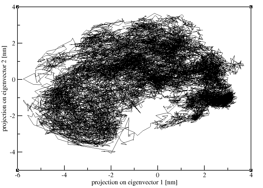
3. Projection of two eigenvectors:

Moreover, we can also calculate the overlap between the principal components (PCs) and the coordinates of the trajectory with gmx anaeig:

gmx anaeig -v eigenvec.trr -f md_protein.xtc -eig eigenval.xvg -s md_protein.pdb -first 1 -last 2 -2d 2dproj_ev_1_2.xvg
(Selection: Twice "Backbone")

Then, we can now project all the proteins coordinates during the trajectory onto this new axis, resulting in a new histogram. We will do this for the first two principal motions. Since PC1 and PC2 are orthogonal (by definition), this should result in a roughly spherical cloud, meaning the motions are uncorrelated.